When a Data Centre Knocks on the Bulk Grid
Twelfth entry in this series, and the start of Act III. The first two acts contrasted a European medium-voltage benchmark (where background operating state dominates, r_load = -0.99) against an Australian low-voltage residential feeder (where rooftop-PV export magnitude inverts the relationship, r_mag = 0.90).
This post opens our third stress test: scaling up from distribution feeders to the bulk wholesale transmission grid. AEMO’s 2026 Electricity Statement of Opportunities (ESOO) records a proposed data-centre connection pipeline of 67 GW across 225 projects in Australia’s National Electricity Market (NEM). When a single commercial facility requests 100 MW to 500 MW at a transmission bus, does event magnitude or the wider grid's operating state govern whether connection-point voltage holds?
The wholesale transmission setup
Everything from the earlier audits carries over: exhaustive AC power-flow verification across every candidate scenario rather than a sample, causal calibration windows, and zero reliance on synthetic heuristics.
What changes is the network model and the physical scale. Rather than an unbalanced 415 V feeder or a 14-bus MV benchmark, the testbed is an open-data AC power-flow model of the eastern Australian NEM transmission network (egrimod-nem topology), spanning 912 nodes across New South Wales and Victoria at 132 kV, 220 kV, 330 kV, and 500 kV.
To test whether the background operating state carries explanatory power, the network was subjected to six season-spanning scenarios derived directly from real half-hourly AEMO operational demand:
- Summer-Peak: 11,128 MW regional demand (air-conditioning stress, high volatility)
- Summer-Mean: 6,645 MW
- Winter-Mean: 7,111 MW (Tasmanian/Victorian heating load)
- Autumn-Mean: 5,898 MW
- Spring-Mean: 5,965 MW
- Spring-Minimum: 4,435 MW (deep solar troughs, high rooftop-PV penetration)
Across New South Wales and Victoria, 16 candidate connection nodes were audited. These included the 12 most electrically remote nodes (ranked by shortest-path series reactance to the regional reference node via Dijkstra's algorithm) plus 4 near-reference control nodes. Crossing these 16 nodes with 10 candidate facility capacities (20 MW to 2,000 MW) across all 6 seasonal states yields 960 full AC Newton-Raphson solves in Pandapower.
The finding: magnitude dominates, and background demand swings don't help
Of the 960 candidate combinations, 547 (57.0%) produced statutory voltage violations (V < 0.95 p.u. or solver non-convergence).
When we fit the solved connection-point voltage against candidate connection magnitude versus background regional demand, the result is unequivocal:
r(magnitude) = 0.5107 vs. r(regional demand) = 0.0904
Event magnitude correlates over 5.6× more strongly with voltage degradation than the network's background operating state.
Even more telling than the correlation coefficients is the violation rate across the seasonal states. Across a massive 2.5× swing in regional grid demand (from 4,435 MW in Spring-minimum to 11,128 MW in Summer-peak), the connection-point violation rate remains completely flat:
| Scenario | Regional Demand (MW) | Violation Rate (%) | |---|---|---| | Spring-Minimum | 4,435 | 56.9% | | Autumn-Mean | 5,898 | 56.9% | | Spring-Mean | 5,965 | 56.9% | | Winter-Mean | 7,111 | 56.9% | | Summer-Mean | 6,645 | 57.5% | | Summer-Peak | 11,128 | 56.9% |
The variation is less than 0.6 percentage points. Whether the wider bulk grid is idling on a mild spring weekend or sweating under summer peak air conditioning has virtually zero impact on whether a 500 MW data centre breaches statutory voltage limits at its connection bus.
Is this an artifact of scenario aggregation? (Gap Closed)
A legitimate critique of the 6-scenario design is that grouping operating states into seasonal statistics might artificially suppress the variance of background load. To test this rigorously, we built an 8× finer continuous-state audit (pipeline/dc_continuous_state_audit.py).
Instead of summary statistics, 48 real, half-hourly settlement timestamps were drawn directly from AEMO historical market data, pairing each candidate connection with real simultaneous system loading. This generated 7,680 full AC power-flow solves:
| Metric | 6-Scenario Audit () | Continuous-Timestamp Audit (N = 7,680) | |---|---|---| | r(magnitude) | 0.5107 | 0.5132 | | r(regional demand) | 0.0904 | 0.1047 | | Non-convergence rate | 44.0% | 43.9% |
The numbers barely moved (+0.0025 and +0.0143). The dominance of connection magnitude over operating state is not an artifact of coarse scenario bins — it is the physical reality of connecting a point-source industrial shock to a transmission corridor.
The physical explanation
Why does background load dictate undervoltage in Germany (r = -0.99) but fail to move the needle here?
In the German medium-voltage benchmark, redispatch adjustments were distributed, modest adjustments (often single-digit MW) evaluated against massive aggregate swings in industrial feeder demand.
A hyperscale data centre, by contrast, is a concentrated point load drawing hundreds of megawatts continuously from a single bus. It represents a massive localized sinkhole in the voltage profile. Because transmission line impedance between the connection point and upstream generation drops voltage in proportion to the transferred power (I · Z), the local voltage drop is overwhelmed by the sheer magnitude of the facility itself. System-wide load diversity cannot rescue a weak connection point from a massive local load.
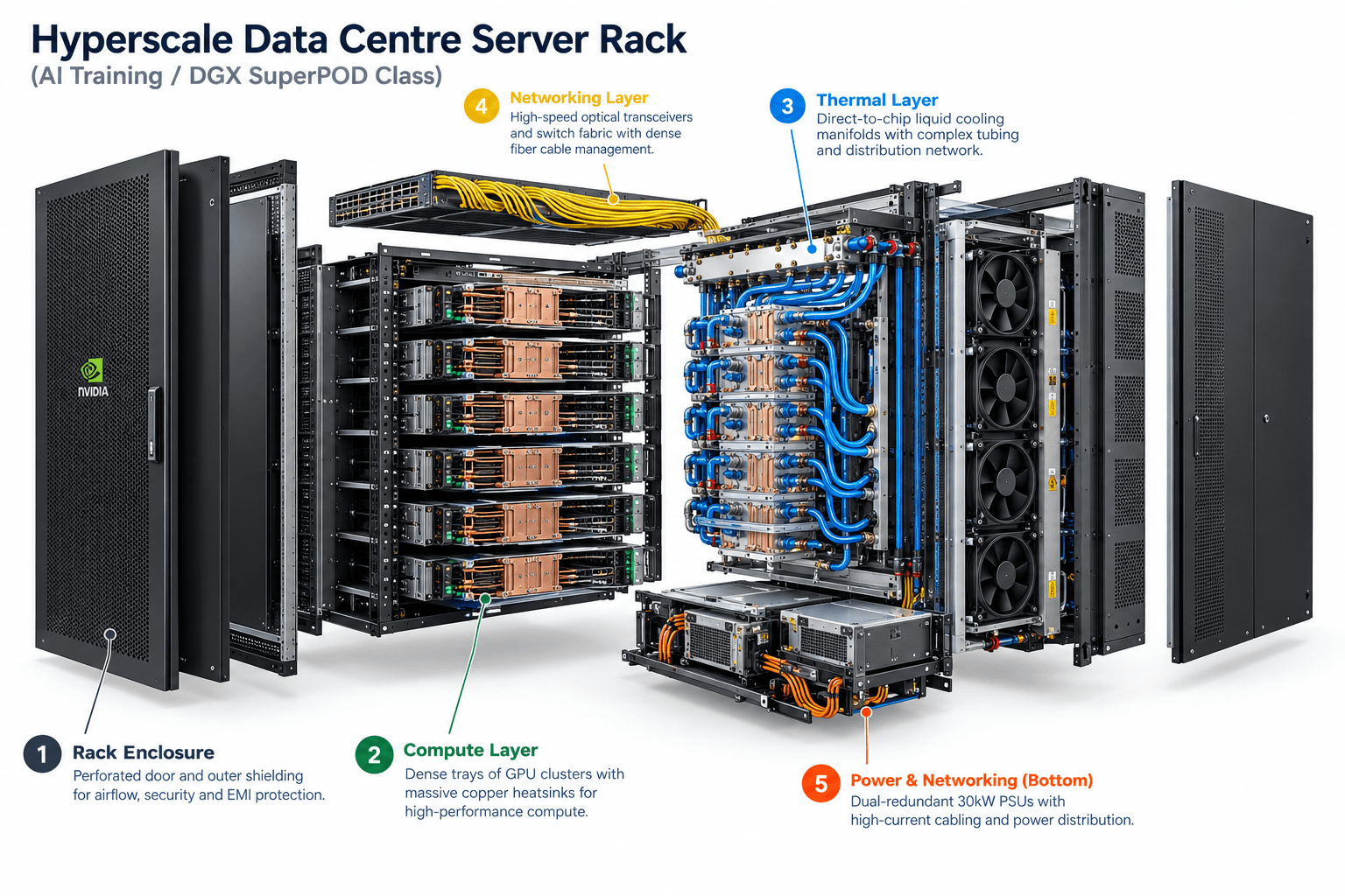
High-Density Data Centre Compute
Hyperscale AI Server Rack
The physical reality of modern cloud computing. Beneath the perforated cabinet lies a dense stack of liquid-cooled GPU clusters, massive dual-redundant 30kW PSUs, and high-throughput optical networking layers.
The unplanned discovery: electrical remoteness
While temporal operating state barely matters, the audit surfaced a second variable that matters enormously: where on the transmission graph the data centre connects.
The 4 near-reference control nodes (nodes with near-zero series reactance to the regional generator slack) experienced exactly zero violations up to 2,000 MW across all 240 combinations tested on them. Meanwhile, electrically remote candidate nodes suffered violation rates between 60% and 90%.
Connecting a data centre to the bulk grid is therefore not a question of when in the year it operates — it is a question of how much it draws, and where on the transmission hierarchy it connects. The next post unpacks that hierarchy: why 500 kV EHV lines easily absorb gigawatt-scale facilities, while 132 kV sub-transmission collapses into physical divergence.
Reproducibility: 960-combination screening audit and continuous-state replay
# Open-data NEM transmission model (egrimod-nem topology in Pandapower)
# 16 candidate nodes (Dijkstra shortest-path series reactance ranked)
# 10 load steps: 20 MW to 2,000 MW (pf = 0.98 near-unity)
# 6 seasonal scenarios from real AEMO regional demand

# Run discrete 960-combination screening audit:
# PYTHONPATH=pipeline python3 pipeline/dc_screening_audit.py
# Result: r_mag = 0.5107, r_load = 0.0904, violation rate flat at ~57%

# Run continuous 7,680-solve audit with real settlement timestamps:
# PYTHONPATH=pipeline python3 pipeline/dc_continuous_state_audit.py
# Result: r_mag = 0.5132, r_load = 0.1047
Full scripts and outputs: pipeline/dc_screening_audit.py, pipeline/dc_continuous_state_audit.py in the data-centre repository.