Engineering Model for Power Grid Strength: Why ShortCircuit Power is the Silent Metric
Smart Grid strength and short-circuit power are the silent constraints shaping HVDC integration.
Published February 3, 2026
Engineering Grid Strength: Why Short‑Circuit Power is the Silent Metric of the Energy Transition ⚡
In my ongoing series on grid resilience—from thermal bottlenecks to fault‑current analysis—I’ve been investigating a hidden risk of the renewable transition: the decline of Short‑Circuit Power (Sk''). As synchronous generators retire, grid strength weakens, making systems more vulnerable to instability during disturbances.
When conducting protection studies, the mathematics of fault calculations determine not just the rating of the switchgear, but the core stability and safety margins of the entire installation. This isn't just theory. I recently conducted a VDE 0102‑compliant short‑circuit study in DIgSILENT PowerFactory, comparing two high‑voltage terminals that could anchor critical infrastructure like the SuedOstLink HVDC corridor.
The Physics of Grid Strength: Short-Circuit Impedance (Uk%)
High-Voltage Step-Down Transformer
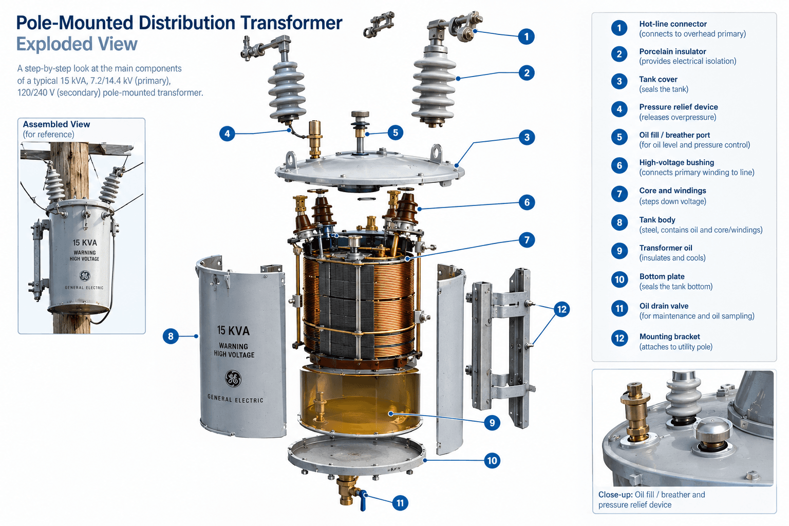
Pole-Mounted Distribution
Engineered for maximum reliability and grid stability. The internal core and windings are suspended in advanced insulating oil, seamlessly stepping down primary transmission voltages to safe, residential levels with built-in overpressure fail-safes.
Before looking at the network-wide data, we have to understand the fundamental physics at the equipment level. When viewing a transformer nameplate, a short-circuit impedance of Uk% = 6% means that if the secondary terminals are short-circuited, exactly 6% of the rated primary voltage must be applied to force full rated current through the windings.
This is the primary mathematical limiter for downstream fault-level calculations. A lower Uk% heavily increases downstream fault intensity.
Live Calculation Example: 1000kVA, 415V, 5% Impedance Transformer
To calculate the maximum symmetric secondary short-circuit current, we first determine the rated secondary current (In):
From Concept to Reality: The 2028 Grid Architecture
Solving grid bottlenecks requires more than theoretical frameworks. Explore our peer-reviewed research and data-driven models that are actively executing these solutions in the field.
Engineering Model for Power Grid Strength: Why ShortCircuit Power is the Silent Metric
Smart Grid strength and short-circuit power are the silent constraints shaping HVDC integration.
Published February 3, 2026
Engineering Grid Strength: Why Short‑Circuit Power is the Silent Metric of the Energy Transition ⚡
In my ongoing series on grid resilience—from thermal bottlenecks to fault‑current analysis—I’ve been investigating a hidden risk of the renewable transition: the decline of Short‑Circuit Power (Sk''). As synchronous generators retire, grid strength weakens, making systems more vulnerable to instability during disturbances.
When conducting protection studies, the mathematics of fault calculations determine not just the rating of the switchgear, but the core stability and safety margins of the entire installation. This isn't just theory. I recently conducted a VDE 0102‑compliant short‑circuit study in DIgSILENT PowerFactory, comparing two high‑voltage terminals that could anchor critical infrastructure like the SuedOstLink HVDC corridor.
The Physics of Grid Strength: Short-Circuit Impedance (Uk%)
High-Voltage Step-Down Transformer
Pole-Mounted Distribution
Engineered for maximum reliability and grid stability. The internal core and windings are suspended in advanced insulating oil, seamlessly stepping down primary transmission voltages to safe, residential levels with built-in overpressure fail-safes.
Before looking at the network-wide data, we have to understand the fundamental physics at the equipment level. When viewing a transformer nameplate, a short-circuit impedance of Uk% = 6% means that if the secondary terminals are short-circuited, exactly 6% of the rated primary voltage must be applied to force full rated current through the windings.
This is the primary mathematical limiter for downstream fault-level calculations. A lower Uk% heavily increases downstream fault intensity.
Live Calculation Example: 1000kVA, 415V, 5% Impedance Transformer
To calculate the maximum symmetric secondary short-circuit current, we first determine the rated secondary current (In):
From Concept to Reality: The 2028 Grid Architecture
Solving grid bottlenecks requires more than theoretical frameworks. Explore our peer-reviewed research and data-driven models that are actively executing these solutions in the field.
Using the transformer's short-circuit impedance (u% = 5%), the maximum prospective short-circuit current (Isc) is:
// Maximum Prospective Fault Current
Isc=u%In=0.051391.2≈27.82kA
In a real-world scenario, accounting for upstream network source impedance, this fault current will typically settle securely inside a 20–25 kA operating bracket. But what happens when we scale this up to the transmission level?
What the Data Reveals: A "Stability Gap"
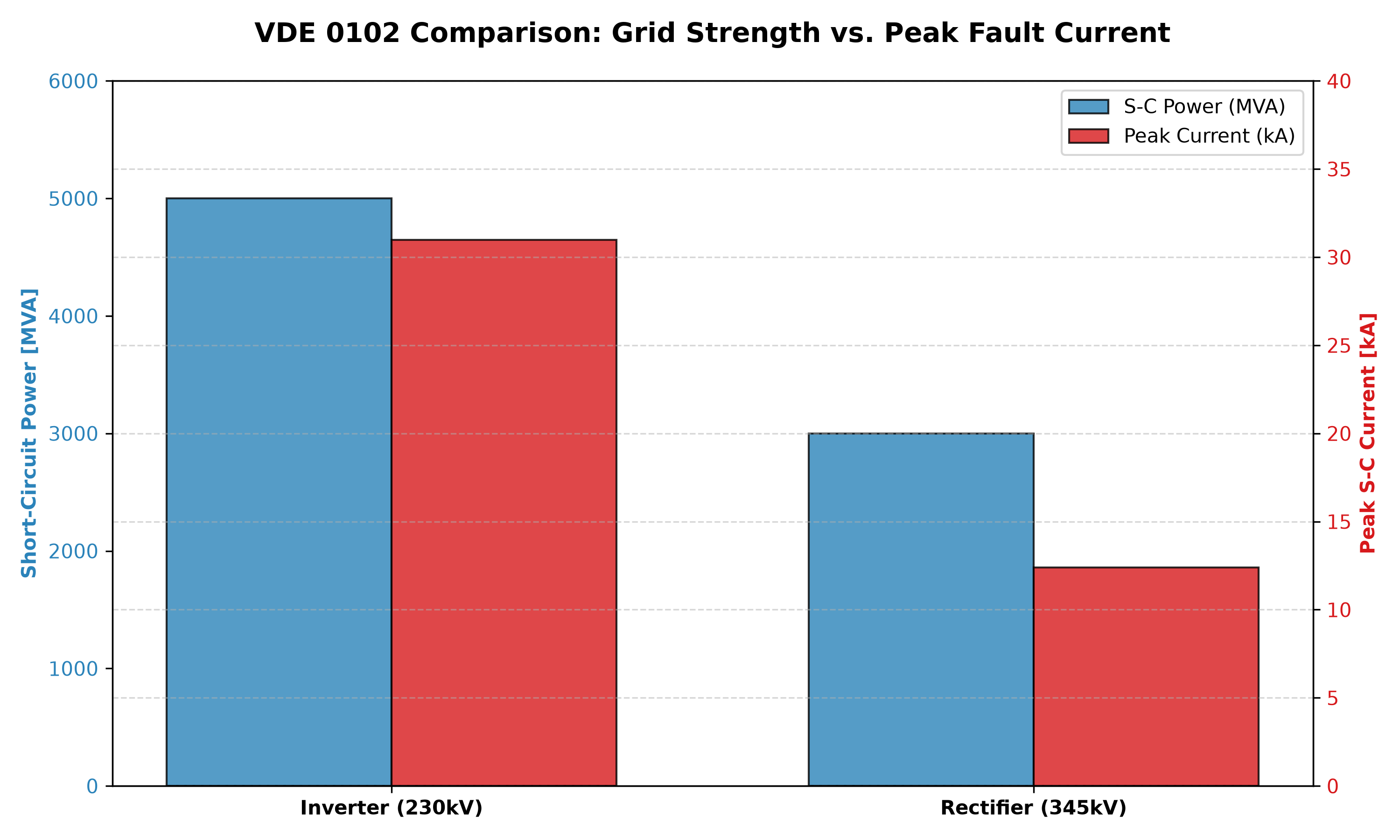
The integration of inverter-based and rectifier-based resources creates distinct short-circuit profiles. The chart below illustrates a comparison of short-circuit power against peak fault currents, modeled via a 0.03 ms Forward-Backward Sweep (FBS) physics solver and DIgSILENT PowerFactory.
Visualizing the "Stability Gap". The Terminal (left) shows significant higher short circuit power (5000 MVA) and peak fault current (30.99 kA) compared to the Rectifier Terminal. This highlights where grid strength must be preserved or enhanced to ensure HVDC stability.
The takeaway: A “strong” grid point (5,000 MVA) provides a robust voltage reference for HVDC links. A “weaker” point (3,000 MVA) could become a vulnerability under high renewable penetration, potentially leading to commutation failures or protection miscoordination.
Protecting the Grid: Coordination and Catastrophe
If grid strength isn't properly managed and fault currents behave unpredictably, protection systems will fail.
ANSI 50 vs. ANSI 51 Protection Coordination
In radial distribution feeder evaluations, ANSI 51 (time-delayed overcurrent protection) is parameterized to ride through transient transformer inrush currents or motor starting spikes, acting as a thermal backup. In contrast, ANSI 50 is the instantaneous overcurrent protection with zero intentional time delay. It is designed to trigger within sub-cycles if a hard, catastrophic line-to-line fault occurs, clearing it instantly before thermal breakdown.
CT Class 5P20 and Saturation Limits
For ANSI 50 to work, Current Transformers (CTs) must accurately relay fault data. A 5P20 rating means the CT has a maximum error of 5% during a massive short-circuit, and it can handle a current 20 times larger than its normal operating limit before magnetically saturating. If a relay receives distorted data due to CT saturation, it might fail to trip.
Arc Flash vs. Normal Arcing
When protection fails, the result is an arc flash—a catastrophic, uncontrolled high-energy fault path through ionized air drawing thousands of amperes. This releases massive incident energy (cal/cm²), requiring strict flash boundaries and PPE category calculations under IEEE 1584 and EN-50110 codes.
From Analysis to Action: Building a Stability‑Aware Digital Twin
To move beyond static compliance checks, I integrated these VDE‑0102 results into a Python‑powered Digital Twin prototype that evaluates grid strength dynamically. The workflow:
VDE‑compliant foundation: PowerFactory automates the fault study, delivering standardized Sk'' and ip values.
Stability analytics: A custom Python layer calculates derived indices (e.g., Short‑Circuit Ratio) and maps them across the network.
Interactive dashboard: A Streamlit interface lets planners simulate contingencies and visualize how reinforcements affect system‑wide strength, not just power flow.
This approach answers the critical question for the 2032 grid: “Does this investment make the grid more resilient, or does it just move the bottleneck?”
Why This Matters for the "60 to 100 by 2032" Mission
The transition isn’t only about adding capacity—it’s about preserving robustness. Tools that link standardized fault studies with interactive planning dashboards help TSOs:
Size switchgear and protection with confidence.
Identify weak nodes before they limit renewable integration.
Turn compliance data into strategic insight.
The Bottom Line
We need Grid‑Stability Architects: engineers who can translate fault currents into resilience strategies, ensuring that a renewable‑powered grid remains as reliable as the one it replaces.
Data Visualization Source Code (Reproducibility)
▼
For reproducibility, the chart above was modeled and rendered using the following Python script. It can be run instantly via uv or directly in a Jupyter Notebook:
Using the transformer's short-circuit impedance (u% = 5%), the maximum prospective short-circuit current (Isc) is:
// Maximum Prospective Fault Current
Isc=u%In=0.051391.2≈27.82kA
In a real-world scenario, accounting for upstream network source impedance, this fault current will typically settle securely inside a 20–25 kA operating bracket. But what happens when we scale this up to the transmission level?
What the Data Reveals: A "Stability Gap"
The integration of inverter-based and rectifier-based resources creates distinct short-circuit profiles. The chart below illustrates a comparison of short-circuit power against peak fault currents, modeled via a 0.03 ms Forward-Backward Sweep (FBS) physics solver and DIgSILENT PowerFactory.
Visualizing the "Stability Gap". The Terminal (left) shows significant higher short circuit power (5000 MVA) and peak fault current (30.99 kA) compared to the Rectifier Terminal. This highlights where grid strength must be preserved or enhanced to ensure HVDC stability.
The takeaway: A “strong” grid point (5,000 MVA) provides a robust voltage reference for HVDC links. A “weaker” point (3,000 MVA) could become a vulnerability under high renewable penetration, potentially leading to commutation failures or protection miscoordination.
Protecting the Grid: Coordination and Catastrophe
If grid strength isn't properly managed and fault currents behave unpredictably, protection systems will fail.
ANSI 50 vs. ANSI 51 Protection Coordination
In radial distribution feeder evaluations, ANSI 51 (time-delayed overcurrent protection) is parameterized to ride through transient transformer inrush currents or motor starting spikes, acting as a thermal backup. In contrast, ANSI 50 is the instantaneous overcurrent protection with zero intentional time delay. It is designed to trigger within sub-cycles if a hard, catastrophic line-to-line fault occurs, clearing it instantly before thermal breakdown.
CT Class 5P20 and Saturation Limits
For ANSI 50 to work, Current Transformers (CTs) must accurately relay fault data. A 5P20 rating means the CT has a maximum error of 5% during a massive short-circuit, and it can handle a current 20 times larger than its normal operating limit before magnetically saturating. If a relay receives distorted data due to CT saturation, it might fail to trip.
Arc Flash vs. Normal Arcing
When protection fails, the result is an arc flash—a catastrophic, uncontrolled high-energy fault path through ionized air drawing thousands of amperes. This releases massive incident energy (cal/cm²), requiring strict flash boundaries and PPE category calculations under IEEE 1584 and EN-50110 codes.
From Analysis to Action: Building a Stability‑Aware Digital Twin
To move beyond static compliance checks, I integrated these VDE‑0102 results into a Python‑powered Digital Twin prototype that evaluates grid strength dynamically. The workflow:
VDE‑compliant foundation: PowerFactory automates the fault study, delivering standardized Sk'' and ip values.
Stability analytics: A custom Python layer calculates derived indices (e.g., Short‑Circuit Ratio) and maps them across the network.
Interactive dashboard: A Streamlit interface lets planners simulate contingencies and visualize how reinforcements affect system‑wide strength, not just power flow.
This approach answers the critical question for the 2032 grid: “Does this investment make the grid more resilient, or does it just move the bottleneck?”
Why This Matters for the "60 to 100 by 2032" Mission
The transition isn’t only about adding capacity—it’s about preserving robustness. Tools that link standardized fault studies with interactive planning dashboards help TSOs:
Size switchgear and protection with confidence.
Identify weak nodes before they limit renewable integration.
Turn compliance data into strategic insight.
The Bottom Line
We need Grid‑Stability Architects: engineers who can translate fault currents into resilience strategies, ensuring that a renewable‑powered grid remains as reliable as the one it replaces.
Data Visualization Source Code (Reproducibility)
▼
For reproducibility, the chart above was modeled and rendered using the following Python script. It can be run instantly via uv or directly in a Jupyter Notebook: